I started this jupyter notebook to help me learn to (1) use both Python and R in one Jupyter notebook and (2) translate tidyverse syntax into Python (specifically pandas & seaborn) syntax. I figured I would post it in the hopes it might be helpful to someone else. Also, I wanted to learn how to post a jupyter notebook on this website.
Helpful links:
Setup
import warnings
warnings.filterwarnings('ignore')
%reload_ext rpy2.ipython
%R library(tidyverse)
array(['bindrcpp', 'dplyr', 'purrr', 'readr', 'tidyr', 'tibble', 'ggplot2',
       'tidyverse', 'tools', 'stats', 'graphics', 'grDevices', 'utils',
       'datasets', 'methods', 'base'],
      dtype='|S9')
# Load in the pandas library
import pandas as pd
import matplotlib.pyplot as plt
import seaborn as sns
%matplotlib inline
Make some fake data
df = pd.DataFrame({'Alphabet': ['a', 'b', 'c', 'd','e', 'f', 'g', 'h','i'],
                   'A': [4, 3, 5, 2, 1, 7, 7, 5, 9],
                   'B': [0, 4, 3, 6, 7, 10,11, 9, 13],
                   'C': [1, 2, 3, 1, 2, 3, 1, 2, 3]})
Glimpse & Summarize
%R glimpse(df)
function (x, df1, df2, ncp, log = FALSE)
df.head()
|
A |
Alphabet |
B |
C |
| 0 |
4 |
a |
0 |
1 |
| 1 |
3 |
b |
4 |
2 |
| 2 |
5 |
c |
3 |
3 |
| 3 |
2 |
d |
6 |
1 |
| 4 |
1 |
e |
7 |
2 |
%%R -i df
summary(df)
       A            Alphabet       B            C
 Min.   :1.000   a      :1   Min.   : 0   Min.   :1
 1st Qu.:3.000   b      :1   1st Qu.: 4   1st Qu.:1
 Median :5.000   c      :1   Median : 7   Median :2
 Mean   :4.778   d      :1   Mean   : 7   Mean   :2
 3rd Qu.:7.000   e      :1   3rd Qu.:10   3rd Qu.:3
 Max.   :9.000   f      :1   Max.   :13   Max.   :3
                 (Other):3
df.info(null_counts = True)
<class 'pandas.core.frame.DataFrame'>
RangeIndex: 9 entries, 0 to 8
Data columns (total 4 columns):
A           9 non-null int64
Alphabet    9 non-null object
B           9 non-null int64
C           9 non-null int64
dtypes: int64(3), object(1)
memory usage: 360.0+ bytes
Filtering
%R df %>% filter(A > 2)
|
A |
Alphabet |
B |
C |
| 1 |
4 |
a |
0 |
1 |
| 2 |
3 |
b |
4 |
2 |
| 3 |
5 |
c |
3 |
3 |
| 4 |
7 |
f |
10 |
3 |
| 5 |
7 |
g |
11 |
1 |
| 6 |
5 |
h |
9 |
2 |
| 7 |
9 |
i |
13 |
3 |
df[df.A > 2]
|
A |
Alphabet |
B |
C |
| 0 |
4 |
a |
0 |
1 |
| 1 |
3 |
b |
4 |
2 |
| 2 |
5 |
c |
3 |
3 |
| 5 |
7 |
f |
10 |
3 |
| 6 |
7 |
g |
11 |
1 |
| 7 |
5 |
h |
9 |
2 |
| 8 |
9 |
i |
13 |
3 |
Slice & Select
%R df %>% slice(4:5)
|
A |
Alphabet |
B |
C |
| 1 |
2 |
d |
6 |
1 |
| 2 |
1 |
e |
7 |
2 |
df.loc[3:4,:] # Note: if slicing only one row, use df.loc[[3],:]
|
A |
Alphabet |
B |
C |
| 3 |
2 |
d |
6 |
1 |
| 4 |
1 |
e |
7 |
2 |
%R df %>% select(A:B)
|
A |
Alphabet |
B |
| 0 |
4 |
a |
0 |
| 1 |
3 |
b |
4 |
| 2 |
5 |
c |
3 |
| 3 |
2 |
d |
6 |
| 4 |
1 |
e |
7 |
| 5 |
7 |
f |
10 |
| 6 |
7 |
g |
11 |
| 7 |
5 |
h |
9 |
| 8 |
9 |
i |
13 |
df.loc[:, "A":"B"] # Select non-adjacent columns with df.loc[:, ["A","B"]]
|
A |
Alphabet |
B |
| 0 |
4 |
a |
0 |
| 1 |
3 |
b |
4 |
| 2 |
5 |
c |
3 |
| 3 |
2 |
d |
6 |
| 4 |
1 |
e |
7 |
| 5 |
7 |
f |
10 |
| 6 |
7 |
g |
11 |
| 7 |
5 |
h |
9 |
| 8 |
9 |
i |
13 |
%R df %>% select(-A)
|
Alphabet |
B |
C |
| 0 |
a |
0 |
1 |
| 1 |
b |
4 |
2 |
| 2 |
c |
3 |
3 |
| 3 |
d |
6 |
1 |
| 4 |
e |
7 |
2 |
| 5 |
f |
10 |
3 |
| 6 |
g |
11 |
1 |
| 7 |
h |
9 |
2 |
| 8 |
i |
13 |
3 |
df.drop(labels = ["A"], axis = 1) # Can use columns = ["A"] in Python 3 / Pandas 0.21.0.
|
Alphabet |
B |
C |
| 0 |
a |
0 |
1 |
| 1 |
b |
4 |
2 |
| 2 |
c |
3 |
3 |
| 3 |
d |
6 |
1 |
| 4 |
e |
7 |
2 |
| 5 |
f |
10 |
3 |
| 6 |
g |
11 |
1 |
| 7 |
h |
9 |
2 |
| 8 |
i |
13 |
3 |
Arrange / Sort
%R df %>% arrange(desc(A))
|
A |
Alphabet |
B |
C |
| 1 |
9 |
i |
13 |
3 |
| 2 |
7 |
f |
10 |
3 |
| 3 |
7 |
g |
11 |
1 |
| 4 |
5 |
c |
3 |
3 |
| 5 |
5 |
h |
9 |
2 |
| 6 |
4 |
a |
0 |
1 |
| 7 |
3 |
b |
4 |
2 |
| 8 |
2 |
d |
6 |
1 |
| 9 |
1 |
e |
7 |
2 |
df.sort_values(by="A", ascending=False)
|
A |
Alphabet |
B |
C |
| 8 |
9 |
i |
13 |
3 |
| 5 |
7 |
f |
10 |
3 |
| 6 |
7 |
g |
11 |
1 |
| 2 |
5 |
c |
3 |
3 |
| 7 |
5 |
h |
9 |
2 |
| 0 |
4 |
a |
0 |
1 |
| 1 |
3 |
b |
4 |
2 |
| 3 |
2 |
d |
6 |
1 |
| 4 |
1 |
e |
7 |
2 |
Mutate
%R df %>% mutate(AoverC = A / C, Bplus1 = B + 1)
|
A |
Alphabet |
B |
C |
AoverC |
Bplus1 |
| 1 |
4 |
a |
0 |
1 |
4.000000 |
1.0 |
| 2 |
3 |
b |
4 |
2 |
1.500000 |
5.0 |
| 3 |
5 |
c |
3 |
3 |
1.666667 |
4.0 |
| 4 |
2 |
d |
6 |
1 |
2.000000 |
7.0 |
| 5 |
1 |
e |
7 |
2 |
0.500000 |
8.0 |
| 6 |
7 |
f |
10 |
3 |
2.333333 |
11.0 |
| 7 |
7 |
g |
11 |
1 |
7.000000 |
12.0 |
| 8 |
5 |
h |
9 |
2 |
2.500000 |
10.0 |
| 9 |
9 |
i |
13 |
3 |
3.000000 |
14.0 |
df.assign(AoverC = df.A / df.C, Bplus1 = lambda df: df["B"] + 1 )
|
A |
Alphabet |
B |
C |
AoverC |
Bplus1 |
| 0 |
4 |
a |
0 |
1 |
4.000000 |
1 |
| 1 |
3 |
b |
4 |
2 |
1.500000 |
5 |
| 2 |
5 |
c |
3 |
3 |
1.666667 |
4 |
| 3 |
2 |
d |
6 |
1 |
2.000000 |
7 |
| 4 |
1 |
e |
7 |
2 |
0.500000 |
8 |
| 5 |
7 |
f |
10 |
3 |
2.333333 |
11 |
| 6 |
7 |
g |
11 |
1 |
7.000000 |
12 |
| 7 |
5 |
h |
9 |
2 |
2.500000 |
10 |
| 8 |
9 |
i |
13 |
3 |
3.000000 |
14 |
To use functions that are NOT vectorized
%%R -i df
is_b <- function(letter) { letter == "b" } # Pretend this function doesn't work on vectors
df %>%
    rowwise %>%
    mutate(is_Alphabet_b = is_b(Alphabet))
Source: local data frame [9 x 5]
Groups: <by row>

# A tibble: 9 x 5
      A Alphabet     B     C is_Alphabet_b
  <int>   <fctr> <int> <int>         <lgl>
1     4        a     0     1         FALSE
2     3        b     4     2          TRUE
3     5        c     3     3         FALSE
4     2        d     6     1         FALSE
5     1        e     7     2         FALSE
6     7        f    10     3         FALSE
7     7        g    11     1         FALSE
8     5        h     9     2         FALSE
9     9        i    13     3         FALSE
def is_b(letter):
    return letter == "b" # Again, pretend not vectorized

df.assign(
    is_Alphabet_b = lambda df: df.Alphabet.apply(is_b)
)
|
A |
Alphabet |
B |
C |
is_Alphabet_b |
| 0 |
4 |
a |
0 |
1 |
False |
| 1 |
3 |
b |
4 |
2 |
True |
| 2 |
5 |
c |
3 |
3 |
False |
| 3 |
2 |
d |
6 |
1 |
False |
| 4 |
1 |
e |
7 |
2 |
False |
| 5 |
7 |
f |
10 |
3 |
False |
| 6 |
7 |
g |
11 |
1 |
False |
| 7 |
5 |
h |
9 |
2 |
False |
| 8 |
9 |
i |
13 |
3 |
False |
Grouping & Summarizing
%%R -i df
df %>%
    group_by(C) %>%
    summarize(avg_A = mean(A), mean_B = mean(B))
# A tibble: 3 x 3
      C    avg_A   mean_B
  <int>    <dbl>    <dbl>
1     1 4.333333 5.666667
2     2 3.000000 6.666667
3     3 7.000000 8.666667
df.groupby("C")\
  .agg({'A' : ['mean'], 'B' : ['mean']})
|
A |
B |
|
mean |
mean |
| C |
|
|
| 1 |
4.333333 |
5.666667 |
| 2 |
3.000000 |
6.666667 |
| 3 |
7.000000 |
8.666667 |
This is super nasty. I hope I can find something better or will need to practice with this a lot.
Joins
First I’ll create a second fake dataset to join
df2 = pd.DataFrame({'Group': ["First", "Second", "Third"],
                   'C': [1, 2, 3]})
%%R -i df,df2
df %>% left_join(df2, by = "C")
  A Alphabet  B C  Group
1 4        a  0 1  First
2 3        b  4 2 Second
3 5        c  3 3  Third
4 2        d  6 1  First
5 1        e  7 2 Second
6 7        f 10 3  Third
7 7        g 11 1  First
8 5        h  9 2 Second
9 9        i 13 3  Third
df.merge(df2, how = "left", on = "C")
|
A |
Alphabet |
B |
C |
Group |
| 0 |
4 |
a |
0 |
1 |
First |
| 1 |
3 |
b |
4 |
2 |
Second |
| 2 |
5 |
c |
3 |
3 |
Third |
| 3 |
2 |
d |
6 |
1 |
First |
| 4 |
1 |
e |
7 |
2 |
Second |
| 5 |
7 |
f |
10 |
3 |
Third |
| 6 |
7 |
g |
11 |
1 |
First |
| 7 |
5 |
h |
9 |
2 |
Second |
| 8 |
9 |
i |
13 |
3 |
Third |
Plotting
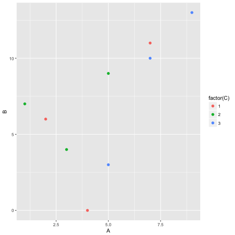
%%R -i df
df %>%
    ggplot() +
    geom_point(aes(x=A, y=B, color=factor(C)), size = 2)
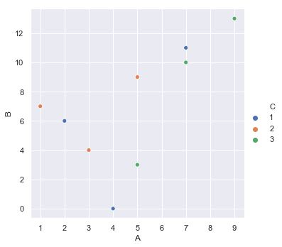
sns.set(style="darkgrid")
sns.relplot(x="A", y="B", hue="C", data=df,
           palette = sns.color_palette(n_colors = 3))
<seaborn.axisgrid.FacetGrid at 0x11cd56e10>